Introduction


FLARES is an online, open-source software for free-list analyses.

FLARES was developed to overcome some of the limitations of its direct ancestor FLAME which is a set of VBA macros running under Microsoft Excel (Pennec et al., 2012).

While maintaining the same philosophy - making free-list analysis as user-friendly as possible - FLARES offers:

  • An extended accessibility. Web-based, you just need a web-browser and you can access FLARES from any operating system.
  • Regular updates. Users are always sure to work with the latest version of FLARES as the application is regularly updated on the server.
  • Integrated statistical analyses. While FLAME required the use of third-party software to conduct exploratory and multivariate analyses, the latter have been directly integrated into FLARES through the use of existing R packages (listed in the 'About' sub-tab).
  • A user-friendly and interactive interface. The use of rStudio's shiny package allows for an interactive interface allowing user's to generate tables and aesthetic plots without ever modifying their original data.

Please visit the other sub-tabs of this 'Introduction' to learn more about FLARES and how to use it.

If you are familiar with R and rStudio you may run FLARES locally on your computer by forking the application on GitHub.


The development of FLARES has been made possible through the support of:

FLARES' development was finalized in 2017 while the main author was funded by a post-doctoral grant awarded by the FYSSEN Foundation.

The idea of developing FLARES sprang within the international research program PIAF (Interdisciplinary Program on indigenous indicators of Fauna and Flora) during which large datasets of free-lists were collected in four different countries (Cameroon, France, USA and Zimbabwe).


Free-listing is a data collection task which was elaborated in the field of cognitive psychology in order to better understand the processes of semantic categorization. Its use has become widespread in the fields of cognitive anthropology, ethnobiology and socio-ecological studies. It is an elicitation technique by which informants are asked to cite - in written or oral form - all the items belonging to a specific super-ordinate semantic category (or cultural domain). A typical question engaging such an elicitation would be:

Please cite, as they come to mind, all the insects that you know of.


This simple data collection technique may be used to:

  • Explore the contents and structure of the investigated cultural domain by:
    • Defining the semantic boundaries of the cultural domain.
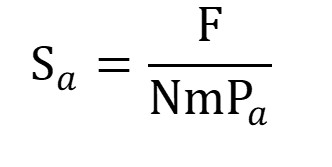
    • Uncovering the most culturally salient items of the domain (based on their frequency of mention across lists and their rank of citation within lists). See Smith & Borgatti (1997) and Sutrop (2001).
    • Estimating inter-item semantic proximity based on the position of any pair of items within respondents' lists. See Henley (1969) & Winkler-Rhodes et al. (2010).
  • Test for the existence of different patterns of response among groups of resondents by:
    • Breaking down cultural salience results by categories of resondents (defined by user).
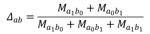
    • Estimating respondents pairwise proximity based on the presence or absence of items within their lists.

Furthemore, the free-listing task may be accompanied by follow-up interviews in which respondents are prompted to provide categorical information concerning the items they have mentioned.

In such cases, statistical tests elaborated by Robbins and Nolan (1997, 2000) enable to test whether respondents:

  • Present a bias in the order in which they mention items belonging to one category or the other (for dichotomous variables).
  • Tend to cluster items in their list based on the category mentioned items belong to.

References:

  • Medical Anthropology Wiki - Free Lists
  • Field Methods Journal
  • Bernard, H. Russell. 2018. Research Methods in Anthropology: Qualitative and Quantitative Approaches. Sixth edition. Lanham, MD: Altamira Press.
  • Borgatti, Stephen P. 1999. 'Elicitation techniques for cultural domain analysis.' In J. Schensul & M. LeCompte (Eds.), Ethnographer's Toolkit, pp.1-26. Walnut Creek: Altamira Press.
  • D'Andrade, Roy G. 1995. The development of cognitive anthropology. Cambridge; New York: Cambridge University Press.
  • Weller, Susan C. & A. Kimball Romney. 1988. Systematic data collection. Newbury Park: Sage Publications.


Most instructions and references to the methods used by FLARES are built into the application and may be found in the different tabs of the application (sub-tabs with details are often named 'Methods').

Below, are provided the few necessary instructions to help you start using FLARES.

1.
Before you can start using FLARES, you must submit an email address in the sidepanel of the 'Introduction' tab.
If you wish to do so, you may submit other information concerning yourself (Name and institution) or your dataset.

You may choose to allow other FLARES' users to access the information you have provided in the 'Users across the globe' sub-tab.

2.
FLARES requires users to upload at least one file:
  • In the 'Upload' tab: you must upload a .csv file containing free-lists, the name/id of respondents and, eventually, categorical information for mentioned items, if provided by respondents.
    Three different input formats are available and are illustrated in the 'Upload' tab.

To benefit from FLARES full capabilities you may also upload two other optional files:
  • In the 'Normalization & Categorization' tab: you may upload a .csv file containing the unique list of all cited items, and as many supplementary columns in which original items may be corrected, translated (i.e. normalization columns) or categorized (i.e. categorization columns).
    The required input format is illustrated in the 'Normalization & Categorization' tab.
  • In the 'Respondent Analyses' tab: you may upload a .csv file containing as many respondent variables as you wish.
    The required input format is illustrated in the 'Respondent Analyses' tab.

N.B. Files that you upload while using FLARES are not stored on the server's hardrive. Uploaded files are used temporarily as long as your session runs. As soon as your session ends, all of your data is cleared from the server's cache memory. However, we do recommend that any data that you upload should be anonymized in order to respect your respondents' privacy.

3.
General guidelines and tips:
  • You may generate your .csv files directly from Microsoft Excel or any other spreadsheet software.
  • When possible, saving your .csv files into UTF-8 encoding is preferred.
  • When possible, avoid special characters as well as periods, slashes or spaces (particularly in the column headings of your files).
  • In the files you wish to upload do not leave header columns blank and do not give identical names to different columns.

All set to go!


FLARES - Free List Analysis under R Environment using Shiny
v 1.0


Fork us on GitHub and access the application's source code:
GitHub Page


Citing FLARES
A paper on FLARES is to be published in a peer-reviewed journal shortly.
Meanwhile, you can cite FLARES as follows:
Wencelius, J., Garine, E., Raimond, C. 2017. FLARES. url:www.anthrocogs.com/shiny/flares/


FLARES is placed under a GNU Affero General Public License v3.0
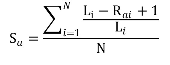
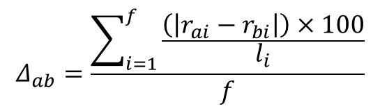
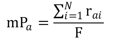


Upload file containing free lists

Normalization and Categorization


You must upload your items list with normalized names or item categories in a .csv or. txt file.

If your data is in an Excel document you can save it as a .csv file before uploading.


No cells should be empty.


Whether it be for normalization or categorization you may create as many columns as you wish (with different headers).

In the table below:

  • The first column contains the items as they are typed-in in the original data.
  • Columns 2 to 4 can be qualified as 'normalization columns'.
  • Columns 5 and 6 can be considered as 'categorization columns'.

Free-List Analyses


Download Free-List Results Table


Download Cultural Salience Chart
Download

Frequency of mention across lists and rank of citation within lists are considered to be good indicators of items relative salience (Bousfield & Barclay 1950).

Two cultural salience indices have been developed to combine these two indicators in order to score each item on a scale ranging from 0 to 1.

Smith Index

The most popular index is Smith's index (Smith and Borgatti 1997; Sutrop 2001).

With:
Sa: Cultural salience of item a
N: Number of lists (number of respondents)
Li: Length of list i
Rai: Citation rank of item a in list i

Sutrop index

Another index was developped by Sutrop (2001) and is less sensitive than the previous with datasets containing lists which length strongly vary from one respondent to the other.

With:
Sa: Cultural salience of item a
N: Number of lists (number of respondents)
F: Frequency of mention of the item across all lists
and mPa: mean rank of citation, with:

With:
rai: rank of citation of item a in list i
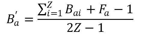
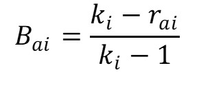
B' score

This measure of cognitive salience, recently developped by Robbins, Nolan and Chen (2017), overcomes some shortcomings of the previous indices, notably:

  • The Smith index does not satisfactorily combine item list position and item frequency as the value of the index will be the same for an item listed once in final position and an item listed last by several respondents.
  • As for the Sutrop index, its minimal value never reaches 0 and the formula involves a computational error for items which are not listed (which is inconvenient when comparing the salience of items across different datasets or subgroups of informants).

The B' score does vary between 0 and 1 and satisfactorily combines both item list position and item frequency.

With:
B'a: Cultural salience of item a
Z: Number of lists (number of respondents)
Fa: Frequency of mention of item a across all lists
and Bai: proportion of items preceding item a in list i given by the following formula:

With:
ki: length of list i
rai: rank of item a in list i


Download Item-by-Item Prox. Matrix Download


Resize plot labels:
Download Item by Item Proximity Plot
Download

When respondents elicit all the known items of a domain they tend to cite similar items in clusters within their lists (Bousfield 1953; Henley 1969).

In consequence, comparing the ranks of citation of any pair of items offers an indication of their semantic proximity.
FLARES offers the possibily to calculate and plot inter-item proximity.

Calculating inter-item proximity

Two methods are used to estimate inter-item proximity.

1. Henley Index: calculates the average difference of citation ranks for every pair of items (Henley 1969),
using the following formula:

With:
Δab: Distance between item a and item b
f: Number of lists in which the pair ab was mentioned
li: Length of list i
rai: Citation rank of item a in list i
rbi: Citation rank of item b in list i

The use of this formula results in the generation of a square item-by-item distance matrix.
This method, however, presents a drawback: two items appearing together in only one list one after the other will have the same distance score as a pair of items appearing in all lists one after the other.
There are two ways to go around this:

  • Discarding items that have been rarely cited (see box concerning plotting of inter-item proximity, below).
  • Using another method to estimate pairwise similarity ('Successive count' presented immediately below).

2. Successive count: counts across lists the number of times a pair of items is mentioned consecutively one after/before the other.
The use of this method is inspired by the works of Brewer (1993) and Romney et al. (1993).

It results in the generation of a square item-by-item contingency table in which cells represent the number of lists in which the corresponding pair of items is mentioned consecutively.
The values in the diagonal are equal to the overall frequency of mention of the corresponding item.

Plotting inter-item proximity

1. Three methods are used to plot inter-item proximity.

  • Correspondance Analysis:
    As suggested by Weller and Romney (1990) correspondance analysis is used to represent into a two-dimensional plot the inter-item proximity derived from the 'Successive count' square contingency table.
    >>'ca' function of the ca R package

  • Multidimensional Scaling (MDS):
    MDS is used to represent inter-item proximity in a two-dimensional plot using the square item-by-item distance matrix computed with the Henley Index.
    >>'cmdscale' function of the basic stats R package

  • Hierarchical Clustering Analysis (HCA - Dendrogram):
    HCA is also used to estimate (and plot as a dendrogram) inter-item proximity.
    >>'hclust' function of the basic stats R package
    >>plot generated with help of: 'dendro_data' function of the ggdendro R package
    • When using the Henley index distance matrix, HCA is performed directly from the latter.
    • When using the 'Successive count' contingency table, HCA is performed on a item-by-item distance matrix computed from the items' coordinates on the main factors of the correspondance analysis mentioned above.

2. Plotting options:

  • Limiting the number of items:
    Exploring inter-item proximity is more robust when looking at the most frequently cited items. For that reason it is possible to limit the number of items to be plotted according to their overall frequency of mention.

  • Displaying item categories:
    If user has uploaded item categorical information he/she may choose to color-code the plot labels according to one of the uploaded items' category (for each category, its sub-categories are plotted with a different color).
    N.B. For item categorical information that was provided by each respondent, each item is assigned to the sub-category which was the most often mentioned for that item. When ties occur (e.g. 10 respondents mentioned they liked the item 'bee' and ten other mentioned they disliked the item 'bee') tie sub-categories (e.g. like_dislike) are created (only for plotting purposes).

Best tree partition

When exploring inter-item proximity through HCA, FLARES offers the possibility to estimate the best partition for items given their position on the dendrogram and given a minimum and maximum number of desired clusters.

The optimal partition is chosen as the one maximizing relative intertia loss. In other words the partition for which clusters are the less heterogeneous.
>>'cutree' function of the dendextend R package

Users may choose to include this 'best' partition for analyses on item categorical information provided in the sub-tab 'Item categories analysis'.


The analyses carried out by FLARES on item categorical information replicate those elaborated by Robbins & Nolan (1997, 2000).

Dichotomous category bias

This analysis is only available for dichotomous variables (e.g. like/dislike, hot/cold, present/absent etc.).

The aim of the analysis is to explore whether items belonging to one of the two sub-categories are more salient than those of the other sub-category.
In order to do so, the idea is to check whether items of one sub-category are more systematically cited early in respondents' lists than the items of the other sub-category.

Robbins & Nolan (1997) designed a score to measure the degree to which respondents cite items with a preferential bias for either sub-categories of a dichotomous variable.

Here are a few details on the score's properties:

  • The score (B) is calculated for each respondent and ranges from 0 to 1 (0 indicating extreme minimum bias, 1 indicating extreme maximum bias and 0.5 inidicating no bias whatsoever).
  • For each respondent the sum of the two B scores (one for each category) is equal to one.
  • The individual B scores may be averaged across the whole sample or sub-groups of the sample.

Assuming that B is normally distributed, a Z-test may be performed in order to test whether the value of the B scores (for the whole sample or sub-groups of the sample) is significantly different from random.
Please refer to the above mentioned paper for details on the methods used to calculate the B score.


What FLARES does:

  • It presents a synthetic table with the B scores averaged across the whole sample.
    If user uploads respondent variables (see 'Respondent Analyses' tab), FLARES breaks down results into sub groups of informants for each respondent variable defined by user.
  • When Z-test is significant, the value of the z statistic is indicated as well as the test's significance level.
  • While the table with the B scores for each respondent is not shown, it may be downloaded.

Semantic category clustering

The aim of this analysis is to test whether respondents tend to elicit items in clusters within their lists. FLARES will test whether items belonging to sub-categories of any given respondent variable (defined by user) are mentioned in clusters by respondents.

Robbins & Nolan (2000) designed a score to measure the degree to which respondents cluster items within their lists.
The score is calculated for each sub-category AND the overarching respondent variable as a whole.

Here are a few details on the score's properties:

  • For each individual the score (C) is calaculated for a given category and each of its sub-categories.
  • C ranges from 0 to 1 (0 indicating minimum clustering, 1 indicating maximum clustering).
  • The individual C scores may be averaged across the whole sample or sub-groups of the sample.

Assuming that C is normally distributed, a Z-test may be performed in order to test whether the value of the C scores (for the whole sample or sub-groups of the sample) is significantly different from random.
Please refer to the above mentioned paper for details on the methods used to calculate the C score.


What FLARES does:

  • It presents a synthetic table with the C scores averaged across the whole sample.
    If user uploads respondent variables (see 'Respondent Analyses' tab), FLARES breaks down results into sub groups of informants as defined by user.
  • When Z-test is significant, the value of the z statistic is indicated as well as test's significance level.
  • While the table with the C scores for each respondent is not shown, it may be downloaded.


Download Data Saturation Plot
Download

Data saturation can be considered as the 'point in data collection and analysis when new information produces little or no change' (Guest et al. 2006).

In order to explore levels of data saturation FLARES seeks to log-fit the number of newly cited items as new respondents are added to the sample.
To optimize the fit, the order of respondents is not random nor does it reflect the order in which respondents appear in users' data files.
Instead, FLARES proceeds as follows:

  • The first respondent is the one with the shortest list.
  • Each new respondent is then chosen to maximize the number of newly cited items.
  • Once the total number of cited items have been accounted for, FLARES stops adding new informants.
  • Finally, FLARES indicates the number of respondents who were needed to account for all items.

While this method poorly represents how free-lists were actually collected, it has the advantage of offering a comparative measure between different datasets.
In fact the ratio of a) number of respondents needed to account for all items to b) total number of respondents may provide an indication of the degree to which the investigated cultural domain is shared.


Respondent Analyses


Download


Download Respondent Competence Chart
Download

Informant competence and cultural centrality

Several indicators computed by FLARES allow to measure each respondent's competence or cultural centrality:

  • List length: number of items mentioned by a respondent.

  • Summed frequency of mentioned items: sum of the overall frequency of mention (across all lists) of the items mentioned by a given respondent.
    N.B. The relation between 'list length' and 'summed frequency of mentioned items' is thought to be linear for culturally central respondents (see 'Informant Competence'/'Chart' sub-tab). Outliers or specialists (i.e. those mentioning a lot of items cited by few other informants) should present a low 'average frequency of mentioned items'.

  • Rank to Frequency correlation: for a given individual it is the value of the R2 coefficient of the Pearson correlation between mentioned items' rank (within the resondent's list) and items' overall frequency (across lists).
    N.B. Culutrally competent or central respondents should present a strong negative correlation coefficient (i.e. they would mention early in their list the most frequently cited items), total outliers should present a strong positive correlation coefficient (i.e. they mention early in their list items mentioned by very few respondents). A negative or positive coefficient close to zero indicates the absence of linear relationship between rank of mention and frequency of citation.


Download Respondent by Respondent Proximity Plot
Download


The table below presents the results (for each respondent variables) of homogeneity of intra-group dispersion across groups.
Homogeneity of dispersion is verified only for variables that have a p-value ABOVE 0.05.

Download

Only the variables for which homogeneity of dispersion is verified are used for the Mulivariate Analysis of Variance presented in the second table (below).
The table below presents the results of the Multivariate Analysis of Variance for each respondent variable presenting a homogeneous intra-group dispersion.
For the variables which have a p-value BELOW 0.05 variation across groups can be considered as significantly higher than variation among groups.

Download

For more details on these analyses, please refer to the 'Methods' sub-tab.


The comparison of patterns of responses (in terms of presence or absence of mentioned items) across respondents allows for the exploration of inter-respondent proximity and for testing for significant variations between sub-groups of respondents (sub-groups of any given respondent variable uploaded by user).

Estimating respondent pairwise similarity

Respondent similarity or proximity is estimated through the use of the Jaccard Index to transform a rectangular binary respondent by item matrix (the value 1 indicates that resondent i has cited item j) into a square respondent by respondent distance matrix (dissimilarity matrix).

The formula for the Jaccard index is the following:


With:
Ma1b0: Number of items which appear in the list of respondent a and not in the list of respondent b.
Ma0b1: Number of items which do not appear in the list of respondent a and do appear in the list of respondent b.
Ma1b1: Number of items which appear in the list of respondent a and appear in the list of respondent b.

Between class analysis

When user uploads respondent variables (e.g. such as gender, age, residence etc.) FLARES offers the possibility to test for significant differences between sub-groups of respondents (e.g. between males and females).
The data used for the test is the square repondent-by-respondent distance matrix described in the box above and the respondent variables uploaded by user in the 'Respondent Analyses'/'Upload' sub-tab.

The test is carried out in two steps (results are displayed in the 'Between Class Analysis' sub-tab):

  • 1. Checking for inter-group homogeneity of intra-group dispersion: for each respondent variable provided by user, an analysis of multivariate homogeneity of intra-group dispersion is carried out.
    >>'betadisper' function of the vegan R package.
    The test's null hypothesis is that between groups there is no difference in levels of intra-group dispersion. In consequence, homogeneity is verified when the test is not significant.
    Only variables for which homogeneity is verified are used in the next step of the analysis
    .

  • 2. Testing for significant differences between groups: a permutational mutlivariate analysis of variance using distance matrices (perMANOVA) is carried out on all respondent variables which intra-group dispersion is homogeneous.
    >>'adonis' function of the vegan R package.

Significant differences in patterns of responses between sub-groups of a respondent variable is verified for variables with a significant p-value at the perMANOVA (see 'Pr(>F)' column of the second table in the 'Between class analysis' sub-tab).

N.B. The results only indicate whether or not there are significant differences between sub-groups, it does not indicate what the differences are. In order to explore how different the patterns of responses are, users may refer to the 'Respondent Analyses'/'Items' saliency' sub-tab in which items' cultural salience scores are broken down by sub-groups of respondents.

Plotting respondent-by-respondent proximity

From the respondent-by-respondent distance matrix (see first box of this page), a Principal Coordinates Analysis (PCoA) is performed in order to generate a two-dimensional plot representing respondent-by-respondent proximity.
>>'dudi.pco' function of the ade4 R package

When user uploads respondent variables, a drop-down list allows user to choose the variable for which sub-groups should be mapped out on the PCoA plot.


Download


Download Free-List Analysis Chart with Respondent Variables
Download
Copyright (C) 2017 Jean Wencélius - GNU License - AGPLv3